Very Short Introduction Plus an Example of Weibull Engineering (WE) Basics

By Wes Fulton, CEO, Fulton Findings (TM)

(originally written 24 JUL 2010, last edited 1 OCT 2021)

The simple concepts in statistics can appear complicated to beginners because many works on the subject use long and strange words. This brief introduction uses shorter and more familiar words. All you need is a healthy curiosity about the way things work.

. . . The pictures in this overview represent some of the many uses for Weibull Engineering (WE) . . .

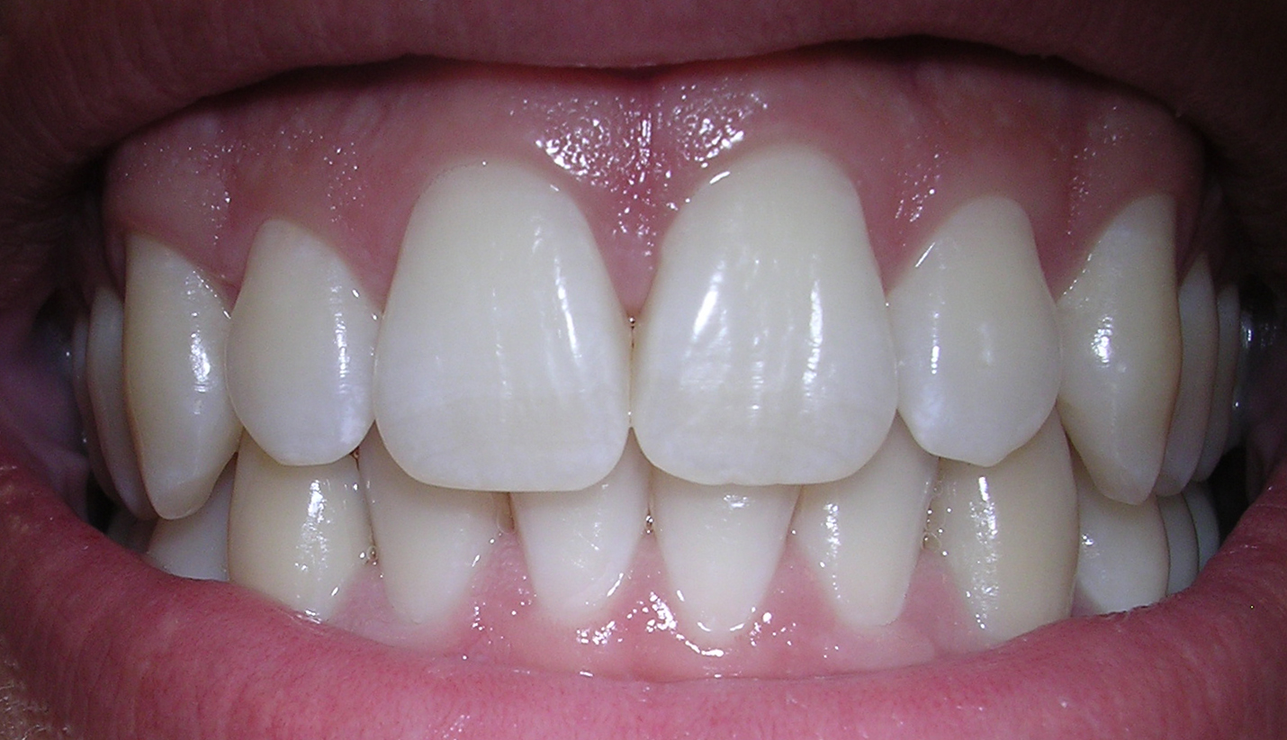
Bearings . . . Aeronautics . . . Physics . . . Automotive . . . Dentistry . . . Welding . . . Gearing

Perhaps the only object without variability is a good digital copy of a digital original. Practically every other product and service has variability. For example, although very similar . . . bearings with the same part number and manufactured one after the other are not going to perform exactly the same. They will have differences in how long they operate successfully. A tiny amount of variability in the type of usage can also make a big difference in operating life capability. Along with lifetime variability, there are other areas where variability effects are important such as money markets, quality satisfaction levels, disease cure rates, satellite reliability, maintenance scheduling, warranty analysis, safety devices, and so on with an almost unending list of additional areas. The good news is that variability can be modeled. Understanding variability and making decisions about variability are straightforward with a proper variability model.

Variability models are called DISTRIBUTIONS. From the correct distribution you can estimate the expected probability of getting a particular result in test or in customer usage. Picking the appropriate model for measurement variability is the entire focus of statistics. In the following, you will notice that a distribution can be presented either as a probability density function (PDF) or a cumulative distribution function (CDF). Those acronyms stand for two different ways to describe the same model . . . but more about that later. There is no math in this introduction, but you can see the math if you want by looking at the references listed at the end.

Exploration . . . Architecture . . . Power Generation and Power Transmission . . . Military . . . Communications

Back around 1920, E.J. Gumbel began to investigate in detail six different EXTREME VALUE distributions for modeling the occurrence of rare events like flooding and wind gusts and power surges. One of these six possible extreme-value distributions is now called the Weibull distribution. It is one of the most widely-used solutions for modeling how things vary, especially for lifetime data (age-to-failure data) and reliability. The name Weibull is usually pronounced in English-speaking countries as WAEE-BULL, but the name is no doubt pronounced differently in Sweden where Waloddi Weibull was born. The subject technique was promoted at first by the technically-gifted Waloddi Weibull. He started investigating variability models (as well as many other things) around 1930 eventually writing over 60 papers plus a book titled Fatigue Testing and Analysis of Results. Weibull`s book was published in 1961 by Pergamon Press [1].

Weibull distribution methods have been frequently updated with an explosion of use since around 1950 and with new applications being added almost continually. Now, there are easy-to-use computer programs available for Weibull modeling along with Weibull classes to teach application. A main reference for this is the handbook by Dr. Bob Abernethy [2]. NOTE: He was `Dr. Bob` before there was `Dr. Who`, `Dr. Dre`, `Dr. Phil`, `Dr. Oz`, etc.

Dr. Bob`s book was the first book written specifically for Weibull Engineering . . . or `WE` . . . and the book is now titled The New Weibull Handbook(C). The first version of it was published in the early 1980`s. It has since been repeatedly updated by Dr. Bob adding the latest methods and describing the latest software solutions to make it the de-facto world standard. Dr. Bob, whose doctorate is in statistics, also invented the engines for the SR-71 Blackbird spy plane! That plane was the eye in the sky for the United States during the post-WWII `Cold War` (from about 1947 to around 1989) between the Eastern Bloc countries and the Western Bloc countries. As of this writing, many decades later and after having been retired, the SR-71 still holds the record as the fastest self-powered manned aircraft with a top speed of 2,269 miles per hour or very near Mach 3. The X-15 and X-43A and Gemini and Apollo capsules and Space Shuttle are technically faster, but those are either not 100% self-powered or not manned. Compare the look of the venerable SR-71 to the futuristic silver-skinned spacecraft in the much later movie Star Wars Episode 1 (released 1999) . . . see the resemblance? Even science fiction loves the all-too-real SR-71 design. The technical expertise of Dr. Bob plus his statistics expertise plus his simple writing style come together to provide good reading, explaining things clearly for practical solutions to real issues. So his book, Reference #2 below, is especially recommended for further reading.

Compared to other commonly used models, the Weibull distribution has a double advantage. One, it is simpler, . . . and two, it is more versatile. It can exactly duplicate distributions like exponential and Rayleigh, and by embracing additional distributions like normal, lognormal, and Type I extreme-value (also called Gumbel after E. J. Gumbel) we get into WE. It has a wider scope than just the analysis of fatigue testing results. WE also includes root-cause detection, event forecasting, spare parts projection, test planning, optimum-replacement for lowest cost, accelerated testing, design comparison, process reliability, manufacturing control, and cost control, as well as others. It currently enjoys wide popularity with many people in the fields of design, development, finance, fabrication, maintenance, operations, quality, reliability, safety, and testing.

Locomotives . . . Electronics . . . Transmissions . . . Machining . . . Food . . . Engines . . . Construction

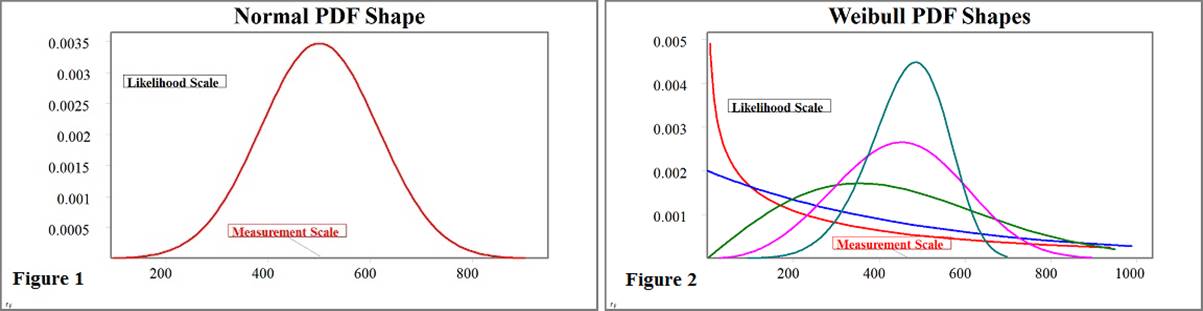
The Normal Distribution: Before some details of the Weibull distribution get presented, let`s look at the well-worn normal distribution. The normal distribution is the king of distributions, modeling many things well . . . but not everything. Waloddi Weibull had an early paper on the Weibull distribution rejected because it was not the normal distribution! The normal distribution probability density function (PDF) has only one basic shape (Figure 1 below) which may be either wider-and-shorter or thinner-and-taller, but it always takes a bell-like shape. It is sometimes called the bell curve, and sometimes called the Gaussian distribution in honor of Johann Carl Friedrich Gauss. The normal distribution applies when modeling variability in such cases as plus/minus error measurements, student test scores, performance variability, X-bar quality control charts, and miss-distance for a machining operation. There is also something called the central limit theorem which explains why the normal distribution fits well when many additive effects are mixed in the data.

The normal distribution model has 2 parameters, meaning that it only requires two numbers for any application. Only the mean value (referred to by the Greek letter Mu, pronounced like mew) and the standard deviation value (Greek letter Sigma) are needed to completely describe a normal distribution. The mean is a central tendency value, representing an expected middle value. Half of the expected values from this distribution are below the mean and half are above. For any symmetrical distribution like normal, the median value (50%) and the mode value (highest PDF point) are the same as the mean value. That is not necessarily true for nonsymmetrical models. The normal distribution standard deviation is a measure of the amount of variability. Higher standard deviation indicates higher variability being measured and also higher variability expected in the future. However, product life and reliability and many real-life measurements need something different.

Life-data measurements exhibit variability not closely symmetrical around a central value. Symmetry around a central value is required for using the normal distribution effectively, and if used incorrectly for reliability purposes the normal distribution can produce negative lifetime estimates. So, the normal distribution is not generally the right choice for modeling lifetime data or age-to-failure measurements for reliability purposes or for that matter not the right choice either for most manufacturing measurements like thickness and surface hardness.

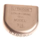
The 2-parameter Weibull: The Weibull distribution works well in modeling lifetime data and most manufacturing data. The Weibull probability density function (PDF) can take many shapes (Figure 2 above) and can fit to non-symmetrical measurements. Also, the simple 1-parameter and 2-parameter versions of the Weibull distribution will not produce a negative value. That is a nice feature for life data analysis and for many actual measurements that cannot be negative. The 2-parameter standard version of Weibull is even simpler than the 2-parameter normal. The math is straightforward for the cumulative Weibull, but the cumulative normal requires higher-math integral approximations . . . UGH!

The standard Weibull is similar in complexity to the normal as it also has only two parameters, characteristic value (referred to by the Greek letter Eta pronounced like ey-tah) and slope value (Greek letter Beta pronounced like bey-tah). Shape parameter is another name for Weibull slope, since the Weibull PDF shape changes with different Beta values. The Weibull slope value moves in opposite direction to variability, such that higher Beta indicates lower variability (desirable for higher quality). Eta is the Weibull version of a central-tendency value. It is approximately near the expected measurement. For some reason, the NIST explanation of Weibull, and the Wikipedia explanation, and the referenced international standard are all as of this writing out-of-step with each other when it comes to Weibull naming convention. Other references may use different parameter names than used here, however Eta and Beta are used for the Weibull 2-parameter distribution in Dr. Abernethy`s handbook [2] and in the international standard, IEC 61649, Edition 2, Weibull Analysis [3].

NOTE: Equations are omitted here for readability, but they are readily available in the recommended references below and in many other references. Table 1 below summarizes some of the reasons the Weibull distribution is gaining in usage.

TABLE 1: Distribution Comparison Green Background = Better

Distribution Model	Normal	Weibull (Standard)
Quantity of Parameters (Complexity . . . Lower is Better)	2	2
Applications	VERY MANY	VERY MANY
Good for Zero and Negative as well as Positive Data (e.g. Residuals, Miss-Distance, etc.)	YES	NO
Good for Data Symmetrical Around a Central Tendency Value	YES	NO
Good for Non-Symmetrical Data	NO . . . Models Well Only Perfectly Symmetrical Measurements	YES
Good for Positive-Only Data Found with Most Manufacturing and Operational Measurements (e.g. Life Data, Cycle Count, Wall Thickness, Case Depth, Performance, Thrust, Altitude, Speed, Braking, Torque, Energy, Pulse Rate, Blood Pressure, etc.)	NO . . . Always Predicts Some Probability of Negative Results	YES
Can Identify Type of Failure Mechanism When Used for Reliability Analysis	NO	YES . . . Weibull Slope (Beta) Can Often Identify Whether Measurements Indicate Infant Mortality or Wear Out
1-Parameter Version Available	NO*	YES
3-Parameter Version Available	NO**	YES
Easy Monte Carlo Simulation	NO . . . Requires Many Lines of Code Executed for Each Repeated Sample Value Generation	YES . . . Requires Only 1 Line of Code Executed for Each Repeated Sample Value Generation
Size Factor Scalability*	NO	YES
Probability Distribution Function (PDF)	Only Bell-Shaped	Infinite Number of Unique Shapes (Changes to Fit Data)
Cumulative Distribution Function (CDF)	Requires Complex Integral Approximation with Numerical Methods	Short Simple Equation (No Approximation Required)
User-Friendly Advanced Mixture Solution Available	NO	YES

* Technically there can be a 1-Parameter Normal distribution with known Sigma, but it is hardly if ever used due to limited scalability. Wallodi Weibull realized that the normal distribution did not calculate correctly for the situation where loads were distributed into different-sized parts. His rationale for using a different distribution (later named for him) was that he needed something that made sense for changing sizes, something that was scalable like the Weibull distribution.

** A 3-Parameter Normal distribution including an extra time-shift (t0) parameter is not useful.

Figures 1 and 2 above represent probability density function (PDF) shapes. All PDF`s (Weibull or normal or whatever) are identical in one respect, i.e. the area underneath any PDF curve is exactly one (1) or 100%. So the PDF represents 100% of where to expect a similar measurement. The amount of area under the PDF curve, to the left of any point along the PDF plot horizontal measurement scale, is the cumulative distribution function (CDF) form. The CDF is simply another way to express the same model. The CDF representation is more useful for answering questions about variability such as . . . How long can a product go with only a specific proportion of failures expected? A Weibull CDF plot is displayed in Figure 3 below for the worked-out example of WE analysis at the end of this introduction.

Weibull often fits to the data better than the normal for some specific applications due to Weibull`s multi-shape capability. The data itself selects the most appropriate Weibull shape for best solution. Weibull also often fits better and works better as a model for small samples. A small sample is taken here to be twenty (20) or less measured occurrence values per Reference #2 below.

The 1-parameter Weibull: With very small sample sizes the Weibull 1-parameter model, also called Weibayes, is the most accurate solution provided there is sufficient and appropriate historical data to help. It works even down to zero occurrences (a VERY small sample indeed!) as long as there are a few non-occurrences (successes for reliability). With a good estimate of the Weibull slope (Beta) already provided from prior experience, the Weibayes solution requires only finding the Weibull characteristic value (Eta). This often produces a simpler and more accurate model.

The 3-parameter Weibull: With a larger sample size, more than 20 occurrences, the more complex 3-parameter version of Weibull becomes very useful for modeling variability. The additional Weibull distribution third parameter (t0 . . . pronounced like tee-zeeroh) represents a time shift for occurrence age variability. The 3-parameter Weibull works well in cases where either there is a delay in the onset of the occurrence mechanism (a failure free period), or the aging process starts before the item officially begins operation (prior deterioration).

Medicine . . . Chemistry . . . Finance . . . Weather . . . anything with variability . . . and that would be more than 99.9999% of everything!

Other Considerations: Knowing the root cause of an occurrence mechanism provides tremendous help in determining corrective action. Sometimes the Weibull solution can suggest the type of root cause given data is generated only from a single root cause. With only one root cause being analyzed the Weibull slope is usually above 1.0 (wear out) or below 1.0 (infant mortality). Mixing different root causes together can complicate the analysis even though there are reasonable solutions available for that (as long as there are only two or three mechanisms and there is a larger quantity of data). Carl Tarum wrote the first easily-accessible software for advanced mixture analysis like this. Mixing many different root cause mechanisms together in the same data set often produces a Weibull solution with Beta slope-value near 1.0 (simplistic assumption of constant occurrence rate, no matter what age) and with a reasonable goodness of fit to the data. However, with many mechanisms mixed together there is additional randomization and loss of resolution. This missing information could otherwise be used to suggest appropriate corrective action. A major recommendation is to focus on one root cause at a time if possible.

Once the basic Weibull model is determined, it can provide the foundation for forecasting like Abernethy Risk. An additional piece of information needed to forecast is the expected usage rate such as the amount of aging experienced per item each month. For example, distance travelled (miles or kilometers) per vehicle per month would be the applicable usage rate for an automotive application. Flight hours per engine per month might be applicable for aircraft as well as patients per hospital room per month for hospitals. Forecasting may be one of the most useful products of WE. Such calculated expectations provide the basis for spare parts requirements and warranty programs.

WE is not limited to the analysis of life data. It is in demand for evaluating process reliability, instrument calibration intervals, economic variability, and quality control. Paul Barringer pioneered the use of WE specifically for process reliability and instrumentation calibration. These methods are extremely popular in the chemical, petro-chemical, and pharma industries. Dennis Keisic was influential in expanding the use of quality methods beyond the normal distribution to include Weibull and lognormal. Weibull or lognormal should be used for quality control monitoring instead of the classically applied normal distribution where that different model is more appropriate. Examples include `Six Sigma` type quality control efforts in plating thickness variability, rotating shaft wobble, progressive deterioration, and contamination level monitoring. These last few applications are not modeled well with the normal distribution as the measurements cannot be negative (normal will always predict some probability of negative results). The standard Weibull and the lognormal distributions are usually more accurate for these manufacturing applications, since they only predict positive measurement values.

WORKED-OUT EXAMPLE

The Issue - Your organization uses hundreds of batteries all of a similar design. These batteries go into a data recording module that cannot be monitored externally with sensors, as the module is buried within a small medical device implanted into cancer patients. The batteries are seldom required and only operate a few seconds at a time, but the life requirement is in hours to minimize chance of failure. When a battery dies, there is loss of data which requires an excessive cost in re-testing and re-analysis to reproduce the desired data. This costly loss of data is happening too often and your management does not like it. Testing on a new sample of seven batteries provides the following operating hours from new to failed state:

130 hours of battery life before failure (Battery #1)

165 hours of battery life before failure (Battery #2)

234 hours of battery life before failure (Battery #3)

252 hours of battery life before failure (Battery #4)

253 hours of battery life before failure (Battery #5)

295 hours of battery life before failure (Battery #6)

389 hours of battery life before failure (Battery #7)

The Goal - Your management wants you to find out how long any particular battery of the same design should be used before replacement if the chance of failure is limited to only 2 percent (%). Plus, you want to be able to defend your decision to management by being conservative in your estimate of life capability.

The Analysis - You plot the battery test data on Weibull CDF scaling. First you sort the data by their values (lowest to highest). You then place the data points on the Weibull plot horizontally by increasing data value, and vertically by increasing failure probability estimated with order statistics. Then you fit a straight line (on this scaling) to the data. NOTE: Good Weibull software will do all of this for you, you just enter the data. The resulting straight line from lower left to upper right is a standard Weibull solution using graphical `rank regression` (rr). Another way to get a solution repeatedly searches for highest data probability, giving a `maximum likelihood estimate` (mle). The resulting plot models the variability of battery life capability. The Weibull CDF plot of the battery test results (Figure 3 below) shows graphical p-value estimate (pve%) of 79.51 for goodness-of-fit. A pve% value can go anywhere from 0 to 100, and a value of 50 is nominal for data sampled from the same distribution used for the plot. A pve% of 10 or higher is usually acceptable. The pve% of 79.51 here is well above average (a good fit!). The plot also indicates type of data (o/s) with 7 occurrences and 0 suspensions. The fit line has Weibull slope Beta of 3.028 (above one). Any Weibull slope above one indicates wear out as the type of occurrence mechanism. Wear out means that older items fail at a relatively faster rate than newer items. The wear out indication for the batteries allows for a useful planned replacement interval. A nominal life capability estimate of 75 hours comes by reading the horizontal value of the fit line where it crosses 2% on the vertical scale (2% failure probability).

This nominal result is not a conservative estimate. A lower estimate line, called a confidence line, was added to the plot for that. The curved confidence line on the plot is a 90% lower estimate of life capability. There are several methods for estimating confidence bounds like this. The code on the plot, W/rr/c%=pv-90, means that the solution for the straight line is Weibull using the rank regression method with lower(-) 90% confidence estimated by Pivotal (pv) Monte Carlo. When read from the lower confidence line, the conservative estimate of life capability goes down to 30 hours (horizontal scale). Note that 2% failure occurrence probability equates to 98% reliability. With additional similar battery test data, the lower confidence line may get closer to the nominal line. This might give an even higher estimate of life capability for the same 98% reliability.

Adding one cost factor for planned replacement (usually at lower cost) and a second cost factor for emergency replacement due to failure (usually at higher cost) would allow a more detailed optimum replacement study to achieve minimum operational cost. It is possible here because the failure mechanism appears to be wear out. Such a cost study is mostly used for non-safety-related items.

The Result - You make a recommendation for a pre-emptive planned replacement of each battery after 30 hours of operation based upon your Weibull analysis. Later you have more testing accomplished, and these results (consistent with before) reduce the uncertainty by adding the latest data to original data thus bringing the conservative lower bound higher and closer to nominal. That initial conservative estimate of 30 hours life is eventually raised to a very comfortable higher operational value. There are very few problems with this battery after your corrective action is implemented. Management likes you. You are promoted, you are happier, and the Weibull estimate for your own life expectancy increases.

CONCLUSIONS

More probability emphasis is coming to such fields as aerospace, energy production, food production, financial markets, medicine, military, oil refining, physics, public safety, and transportation. WE and similar probability-centered analysis, like Reliability Centered Maintenance (RCM), lead the way in providing useful answers to difficult questions. For more information visit http://www.WeibullNews.com on the web, and view the references at the end.

If you actually read through all of this and it clicked with you, you might be smarter than you think. Quantum physics (not an easy topic) is practically 100% based on probability stuff somewhat similar to this. Rocket scientists and brain surgeons of the world . . . eat your heart out!

REFERENCES

1. Weibull, Waloddi, Fatigue Testing and Analysis of Results, Pergamon Press, 1961 (the only book by Weibull)

2. Abernethy, Robert B. (Dr. Bob), The New Weibull Handbook(c), self-published (first complete self-study reference for Weibull Engineering) . . . here is the link for it on AMAZON:

https://www.amazon.com/dp/0965306232/

3. IEC 61649, Edition 2, Weibull Analysis (the official international standard) . . . here is a link for it: https://webstore.iec.ch/publication/5698

4. Select Here for the SAE Introduction to Weibull Solution Methods

ABOUT THE AUTHOR

Wes Fulton wrote the first widely-used software for WE. He presents Dr. Bob`s Weibull Workshop for organizations and companies and sometimes even for much-maligned governments around the world including their military. He has two engineering degrees and a patent to his name. He writes books for adults and for children.